2 Passive IC devices
Basic Electrostatic and Magnetostatic laws namely: Gauss’ Law, Faraday’s Lay, Ampere’s Law, Coulomb’s Law and Biot-Savart’s Law.
2.1 Introduction
This chapter provides a concise review of passive devices—resistors, capacitors, and inductors—as implemented in integrated circuits (ICs). It is specifically tailored for IC designers, including electrical engineering graduates seeking a refresher and practicing engineers aiming to reinforce their fundamental knowledge. The content balances theoretical underpinnings with practical considerations relevant to modern IC design. Exercises and examples are included to enhance understanding and facilitate application of the concepts discussed.
2.2 Resistance
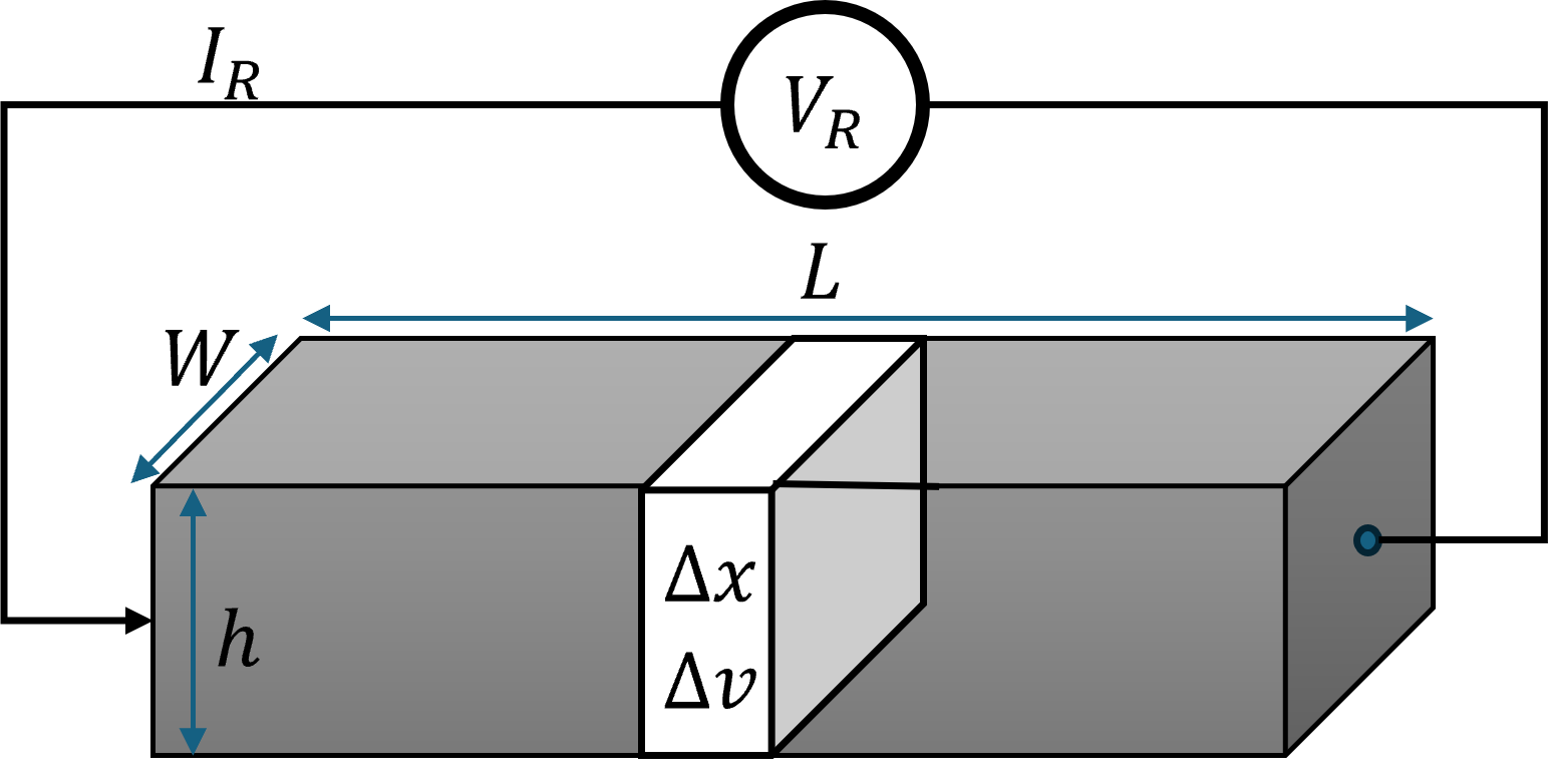
Resistance calculation of metal or semiconductor material is fundamental to IC engineering. Consider a block of metal or semiconductor material with dimensions \(L, W\) and \(h\) as shown in Figure 2.1. Let \(n\) be the charge per unit volume. To calculate the current \(I_R\) for an applied voltage \(V_R\) across the length of the material, we will consider an incremental cross section of the material with length \(\Delta x\). The current can be written as the total charge in the incremental volume in time \(\Delta t\):
\[ I_R = \frac{\Delta Q}{\Delta t} = \frac{Q_S \Delta x}{\Delta t} = Q_S v_d \]
or,
\[ I_R = Sheet Charge \times Average Velocity \]
where, \(Q_S = nWh\) is the sheet-charge or the charge per unit length,
\(v_d\) is the average velocity of the electrons:
\[ v_d= \frac{\Delta x}{\Delta t} = \mu E \]
where, \(E = \frac{\Delta v}{\Delta x}\), and \(\mu\) is the mobility of the material.
Therefore,
\[ I_R = \mu Q_S \frac{\Delta v}{\Delta x} \]
Using Ohm’s law, the incremental resistance can be expressed as
\[ \Delta R = \Delta v / I_R = \rho \frac{\Delta x}{W h} \]
where, \(\rho = 1/(n \mu)\) is the Specific resistivity (\(\rho\)) is a property of the material that can be defined as the resistance per unit volume expressed in SI units of \(\Omega m\) but more conveniently as \(\Omega cm\).
The total resistance of the volume can be found by summing up all incremental resistances \(\Delta R\):
\[ R = \rho \frac{L}{A} \]
where, \(L\) is the length and \(A\) is the cross-sectional areai (\(W h\)).
In integrated circuit design, the height of the metal routing is fixed and is typically in the range of \(0.1\) to \(5\) micrometers (\(\mu m, 10^{-6} m)\) and the resistance is measured in square units as ohms per square or \(\Omega/\square\).
\[ R = (\rho/h) (L/W) \]
Where, \(\rho/h\) is typically called sheet-rho (\(\rho_{sheet}\))
The specific resistance (in \(\Omega cm\)) and unit resistance (in \(\Omega/\square\)) of typical metals used in integrated circuits such as aluminum (Al), copper (Cu) and gold (Au) are tabulated:
| \(\mu -\Omega\) cm | \(m\Omega/\square\) | |
|---|---|---|
| Al | 2.65 | 26.5 |
| Cu | 1.68 | 16.8 |
| Au | 2.44 | 24.4 |
Update material properties of the 3 metals in Table Table 2.1 with melting point, temperature coefficient, and cost in INR for 10gm.
Calculate the resistance of an aluminum wire with the following dimension:
\(L=100\mu m, W=1\mu m, h=0.5\mu m\)
Hint: Re-calculate \(\rho_{sheet}\) from table Table 2.1 and use it to calculate the resistance.
Calculate the sheet-rho(\(\rho_{sheet} ( \Omega/\square\)) and the specific resistivity (\(\rho (\Omega cm\)) for a material with the following dimensions:
\(L=50\mu m, W=1\mu m, h=0.5\mu m\)
and the measured resistance across the length is \(35 \Omega\).
Using a Virtual Laboratory, for example PhET, interactively predict and verify how resistance changes with each parameter (\(\rho, L, A\)). Enter the resistivity of Aluminum, copper and gold, verify the resistance matches your calculation.
2.3 Capacitance
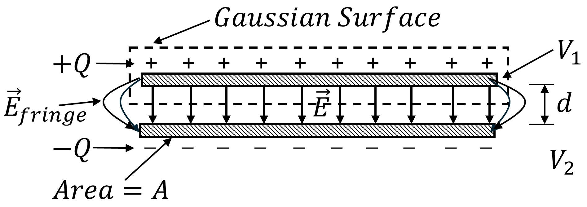
Consider two parallel metal plates of area \(A\) separated by distance \(d\) as shown in Figure 2.2 .
If the total charge on the top and bottom plate is \(+Q\) and \(-Q\) respectively, and the potential on the plates are \(V_1\) and \(V_2\) respectively, total charge on the plate is directly proportional to the potential difference (\(V=V_1-V_2\)):
\[ Q \propto V \]
And the proportionality constant is the capacitance \(C\) of the parallel plates:
\[ Q = CV \]
In order to calculate the capacitance of the parallel plates, we will apply Gauss’ law (\(\nabla\cdot \vec{E} = \rho /\epsilon_0\)) by enclosing the top plate (or bottom plate), as show in Figure 2.2 and calculate the total electric field diverging from the enclosed volume.
Assuming a large area and a small separation, the peripheral electric field can be neglected and average electric field \(\vec{E}\) can be expressed as:
\[ \vec{E} = \frac{V}{d} \]
Applying Gauss’s to find the divergence of \(\vec{E}\):
\[ \int \vec{E}\cdot da = \frac{Q}{\epsilon_0} \]
The flux leaving the bottom surface integrated results in:
\[ EA = \frac{V}{d}A = \frac{Q}{\epsilon_0} \]
Therefore, the capacitance of the parallel plates can be expressed as:
\[ C = \frac{A\epsilon_0}{d} \]
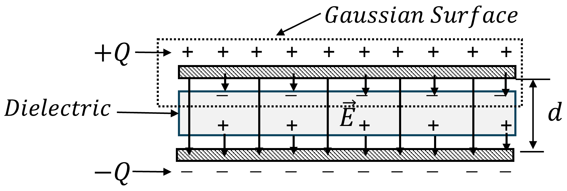
In the presence of dielectric material, as shown in Figure 2.3, the capacitance is expressed as:
\[ C = \frac{A (1+\chi)\epsilon_0}{d} = \frac{A\kappa \epsilon_0}{d} \]
where, \(\chi\) is the dielectric susceptibility and \(\kappa\) is the relative permittivity.
2.4 Inductance
Inductors are virtually nonexistent in Integrated Circuits due to the very small loop areas. Our discussion will be confined to the self-inductance of a current loop to familiarize the reader with the fundamental concepts of self-inductance.
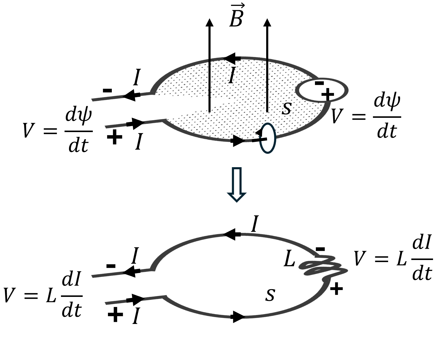
Faraday’s law of induction is crucial for understanding inductance. Consider the circular wire loop in Figure 2.4 , with a small gap for introducing current \(I\). This current circulates counter-clockwise around the loop, as in Figure 2.4 , creating a magnetic flux density \(B\) through the surface \(s\) the loop encloses. The surface’s shape doesn’t affect the result, as long as the loop encircles it. With counter-clockwise current, the magnetic field is upward through the surface. The total magnetic flux through the loop can be calculated as
\[ \psi = \int_S \vec{B}\cdot ds \]
where \(s\) is the surface enclosed by the current loop. If the current and magnetic field change over time, Faraday’s law of induction states that the change in magnetic flux through the loop induces an electromotive force (emf) around its contour.
\[ emf = \int_C \vec{E}\cdot dl = - d\psi / dt \]
where \(C\) is the loop’s contour around surface \(s\). If the loop is electrically small, we can represent the emf as a voltage source equal to the rate of change of magnetic flux through the loop:
\[ V = d\psi / dt \]
Lenz’s law clarifies that the negative sign in Faraday’s law indicates the induced emf and current oppose the change in magnetic flux that creates them. Thus, the voltage source polarity is as shown in Figure 2.4 . Inductance is fundamentally the ratio of the magnetic flux through the loop to the current causing it
\[ L=\frac{\psi}{I} \]
or
\[ \psi = LI \]
In a linear, homogeneous, and isotropic medium, the magnetic flux through the loop is proportional to the current \(I\) that generates it, with inductance as the proportionality constant linking \(I\) and \(\psi\). Therefore, inductance depends solely on the loop’s shape, dimensions, and the medium’s material properties. The induced voltage source is expressed as
\[ V=\frac{d\psi}{dt} \]
or
\[ V=L\frac{dI}{dt} \]
Figure 2.4 illustrates replacing the induced source with an inductor symbol, where the voltage across it is given by \(L\cdot dI/dt\) and appears as a Thevenin open-circuit voltage. If the loop’s wire has resistance, it’s shown with a resistor symbol in series, adding an IR voltage drop around the loop.
The technique used to determine the inductance of a loop is known as the method of flux linkages, as it involves calculating the flux that “links” with the current. This method comprises four steps:
- Injecting a current \(I\) around the closed loop.
- Use Biot-Savart’s law to find the magnetic flux density \(\vec{B}\) over the loop’s surface, akin to Gauss’ law for magnetism.
- Determine the overall magnetic flux passing through the loop by utilizing the equation \(\psi = \int_S \vec{B} \cdot ds\).
- Divide that flux by the current I to get the inductance of the loop.
The inductance so obtained is referred to as the self inductance of the loop.
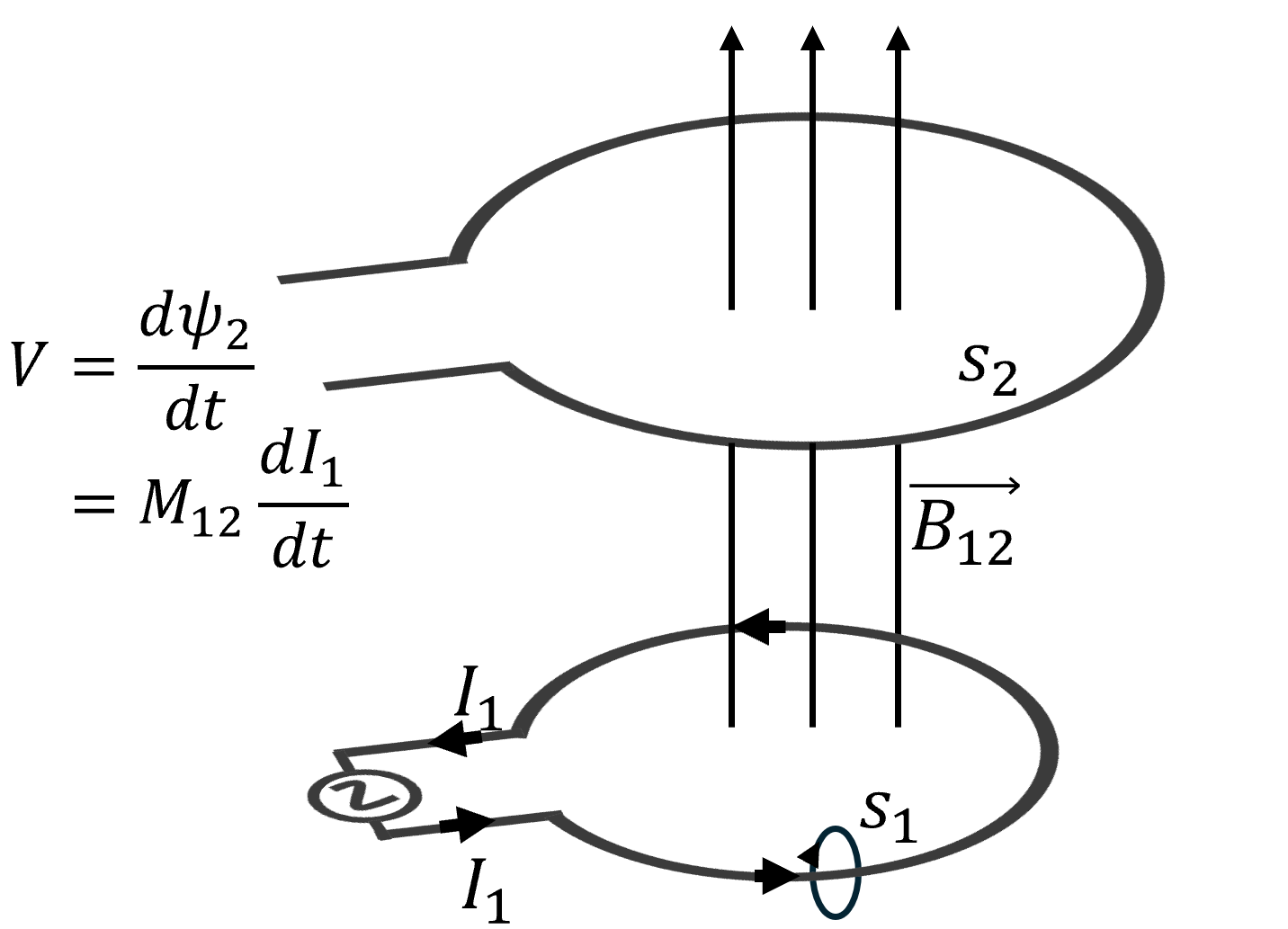
The mutual inductance between two loops, one of which carries a current \(I_1\), is defined with reference to Figure 2.5 as
\[ M_{12} = \frac{\psi_2}{I_1} \]
where \(\psi_2\) is the flux penetrating the surface of the second loop, \(s_2\), that is caused by the current of the first loop:
\[ \psi_2 = \int_{s2} \vec{B}_{12}\cdot ds \]
The determination of the magnetic flux density \(\vec{B}\) can be performed using several approaches, all of which necessitate the computation of complex integrals. To finalize the calculation of the structure’s inductance via the flux linkage method, it will be essential to compute additional intricate integrals involving these \(\vec{B}\) fields.
There are many textbooks that discuss various methods for their calculation, and one such source is Paul (2011) .